
教科書p.60[事例5-b]の分析
回帰式を求め,データと共に描画します.
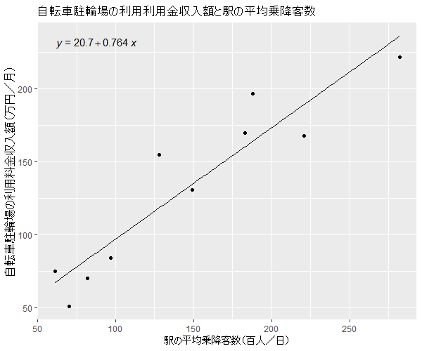
これを描くRのコードは以下です.
# coded by F.Nakai
# 2021.01.20

#データの読み込み
SIU <- read.csv("https://fnakai.web.nitech.ac.jp/data/13_LP/StationIncomeAndUsers.csv")

#Rのlm関数による回帰パラメータの導出
result <- lm(SIU$Income~SIU$UsersNum)
result

##問2 手計算の過程の再現
#yの偏差
yy <- (SIU$Income-mean(SIU$Income))
#xの偏差
xx <- (SIU$UsersNum-mean(SIU$UsersNum))

#xの分散とxとyの共分散を求める
Sxy <- sum(xx*yy)*(1/length(xx))
Sxx <- sum(xx^2)*(1/length(xx))

# b=(xとyの共分散/xの分散)
b <- Sxy/Sxx

# a= (yの平均)-b*(xの平均)
a <- (mean(SIU$Income))-(b*mean(SIU$UsersNum))

#教科書p.61の図を描く
plot(SIU$UsersNum,SIU$Income,
     xlim = c(0,300),
     ylim = c(0,250),
     main = "自転車駐輪場の利用利用金収入額と駅の平均乗降客数",
     xlab = "駅の平均乗降客数(百人/日)",
     ylab = "自転車駐輪場の利用料金収入額(万円/月)"
)

#回帰直線を重ねる
abline(a = a, b = b)

##発展編:きれいに図を描くggplotパッケージの利用

#パッケージのインストール
install.packages("ggplot2")
install.packages("ggpmisc")

#パッケージの読み込み
library(ggplot2)
library(ggpmisc)

#回帰のモデル式を保存しておく
my.formula <- y ~ x

#図を描く
ggplot(data = SIU, mapping = aes(x = UsersNum, y = Income)) +
  geom_point() +
  labs(title = "自転車駐輪場の利用利用金収入額と駅の平均乗降客数") +
  xlab("駅の平均乗降客数(百人/日)") +
  ylab("自転車駐輪場の利用料金収入額(万円/月)") +
  geom_point() +
  geom_smooth(method = "lm", se=FALSE, color="black", formula = my.formula, size = 0.5)+
  stat_poly_eq(formula = my.formula,
               aes(label = paste(..eq.label..)),
               parse = TRUE) +
  theme_gray()

#問2 Table3の計算
table3 <-cbind(SIU,yy,xx,yy^2,xx^2,xx*yy)
table3

##問3 決定係数を求める
#yの予測値からの偏差平方和の平均(配布資料の2.2式)
Sxy2 <- (1/length(SIU$Income))*sum((SIU$Income - predict(result))^2)
Sxy2

#yの分散
Syy <- sum(yy^2)*(1/length(yy))
Syy

#決定係数
r2 <- 1-(Sxy2/Syy)

#相関係数
r <- sqrt(r2)

#Rのlm関数によって求めた決定係数との比較:summary関数を用いた表示
summary(result)

#Rのcor関数によって求めた相関係数との比較
cor(SIU$Income,SIU$UsersNum)